Machine Learning with Mixed Numeric and Nominal Data using COBWEB/3

Demonstration of two extensions to the cobweb/3 algorithm that enables it to better handle features with continuous values.

Problem Overview

Many machine learning applications require the use of both nominal (e.g., color=”green”) and numeric (e.g., red=0, green=255, and blue=0) feature data, but most algorithms only support one or the other. This requires researchers and data scientists to use a variety of ad hoc approaches to convert troublesome features into the format supported by their algorithm of choice. For example, when using regression based approaches, such as linear or logistic regression, all features need to be converted into continuous features. In these cases, it is typical to encode each pair of nominal attribute values as its own 0/1 feature. It is also typical to use one-hot or one-of-K encodings for nominal features. When using algorithms that support nominal features, such as Naive Bayes or Decision Trees, numerical features often need to be converted. In these cases, the numerical features might be converted into discrete classes (e.g., temperature = “high”, “medium”, or “low”). When converting features from one type to another their meaning is implicitly changed. Nominal features converted into numeric are treated by the algorithm as if values between 0 and 1 were possible. Also, some algorithms assume that numeric features are normally distributed and nominal features converted into numeric will follow a binomial, rather than normal, distribution. Conversely, numeric features converted into nominal features lose some of their information.

Luckily, there exist a number of algorithms that support mixed feature types and attempt to balance the different types of features appropriately (usually these are extensions of algorithms that support nominal features). For example, Decision Tree algorithms are often modified to automatically support median split features as a way of handling numeric attributes. Also, Naive Bayes has been modified to use a Gaussian distribution for modeling numeric features. Today I wanted to talk about another algorithm that supports both numeric and nominal features, COBWEB/3.

COBWEB Family of Algorithms

Over the past year Erik Harpstead and I have been developing python implementations of some of the machine learning algorithms in the COBWEB family (our code is freely available on GitHub). At their core, these algorithms are incremental divisive hierarchical clustering algorithm that can be used for supervised, semi-supervised, and unsupervised learning tasks. Given a sequence of training examples, COBWEB constructs a hierarchical organization of the examples. Here is a simple example of a COBWEB tree (image from wikipedia article on conceptual clustering):

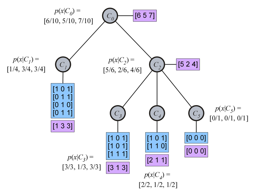
Each node in the hierarchy maintains a probability table of how likely each attribute value is given the concept/node. To construct this tree hierarchy, COBWEB sorts each example into its tree and at each node it considers four operations to incorporate the new example into its tree:

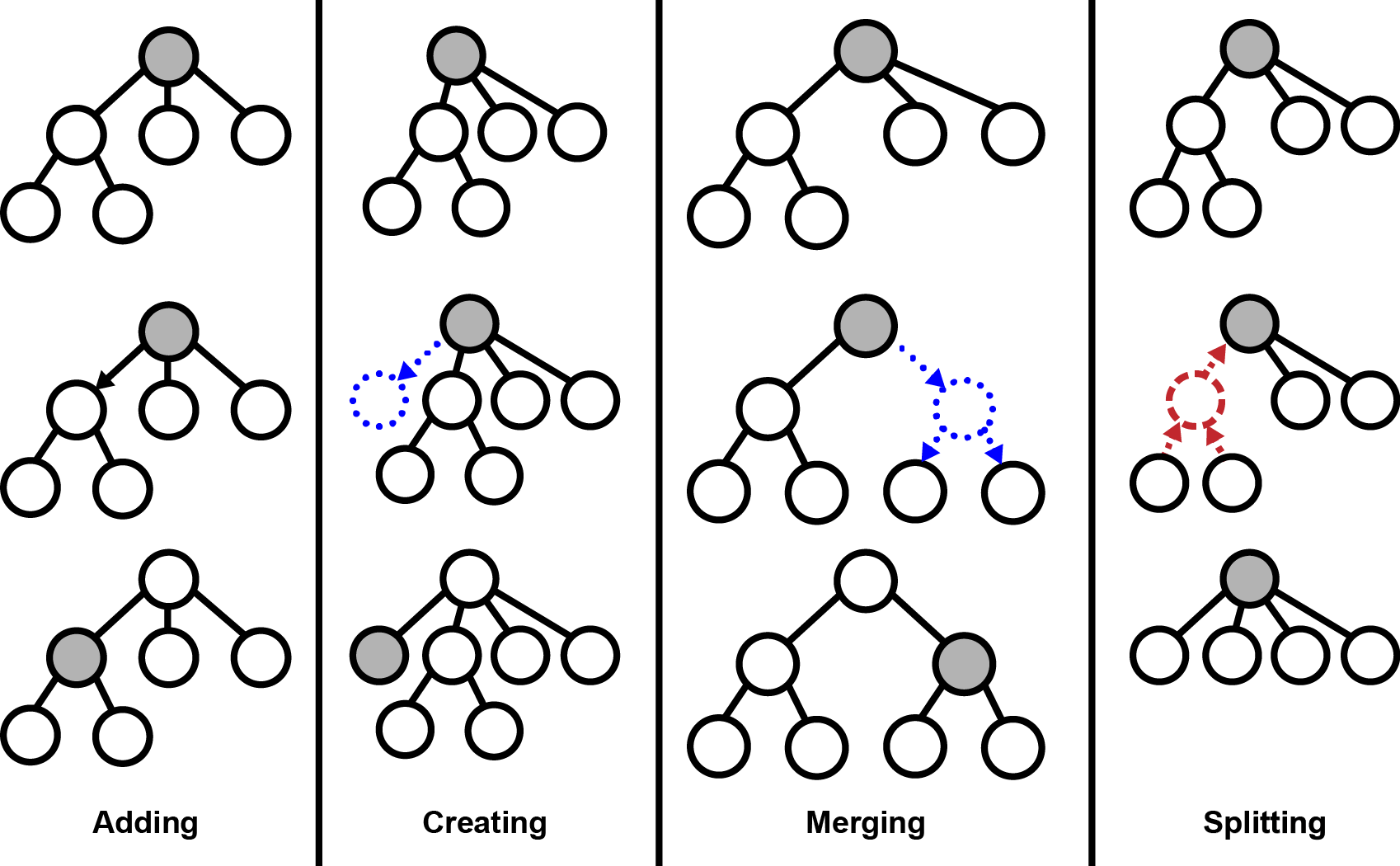
To determine which operation to perform, COBWEB simulates each operation, evaluates the result, and then executes the best operation. For evaluation, COBWEB uses Category Utility:

\[CU({C_1, C_2, ..., C_n}) = \frac{1}{n} \sum_{k=1}^n P(C_k) \left[ \sum_i \sum_j P(A_i = V_{ij} | C_k)^2 - \sum_i \sum_j P(A_i = V_{ij})^2 \right]\]

This measure corresponds to increase in the number of attribute values that can be correctly guessed in the children nodes over the parent. It is similar to the information gain metric used by decision trees, but optimizes for the prediction of all attributes rather than a single attribute.

Once COBWEB has constructed a tree, it can be used to return clusterings of the examples at varying levels of aggregation. Further, COBWEB can perform prediction by categorizing partially specified training examples (e.g., missing the attributes to be predicted) into its tree and using its tree nodes to make predictions about the missing attributes. Thus, COBWEB’s approach to prediction shares many similarities with Decision Tree learning, which also categorizes new data into its tree and uses its nodes to make predictions. However, COBWEB can be used to predict any missing attribute (or even multiple missing attributes), whereas each Decision Tree can be used to predict a single attribute.

COBWEB’s approach is also similar to the k-nearest neighbors algorithm; e.g., it finds the most similar previous training data and uses this to make predictions about new instances. However, COBWEB uses its tree structure to make the prediction process more efficient; i.e., it uses its tree structure to guide the search for nearest neighbors and compares each new instance with \(O(log(n))\) neighbors rather than \(O(n)\) neighbors. Earlier versions of COBWEB were most similar to nearest neighbor \(k=1\) because they always categorized to a leaf and used the leaf to make predictions, but later variants (which we implement in our code) use past performance to decide when it is better to use intermediate tree nodes to make predictions (higher nodes in the tree correspond to a larger number of neighbors being used). Thus, with less data, COBWEB might function similarly to nearest neighbors, but as it accumulates more data it dynamically adapts the number of neighbors it uses to make predictions based on past performance.

COBWEB/3

Now returning to our original problem, the COBWEB algorithm only operates with nominal attributes; e.g., a color attribute might be either “green” or “blue”, rather than a continuous value. The original algorithm was extended by COBWEB/3, which modeled the probability of each numeric attribute value using a Gaussian distribution (similar to how Naive Bayes handles numeric data). With this change, i.e., \(P(A_i = V_{ij} | C_k)^2\) is replaced with \(\frac{1}{2 * \sqrt{pi} * \sigma_{ik}}\) and \(P(A_i = V_{ij})^2\) is replaced with \(\frac{1}{2 * \sqrt{pi} * \sigma_{i}}\) for continuous attributes. I find COBWEB’s approach to handling mixed numeric and nominal attributes interesting because it treats each as what they are (numeric or nominal), but combines them in a principled way using category utility. This approach is not without problems though. I’m going to talk about two problems with the COBWEB/3 approach and how I have overcome them in my COBWEB/3 implementation.

Problem 1: Small values of (sigma)

This approach runs into problems when the \(\sigma\) values get close to 0. In these situations \(\frac{1}{\sigma} \rightarrow \infty\). To handle these situations, COBWEB/3 bound \(\sigma\) by \(\sigma_{acuity}\), a user defined value that specifies the smallest allowed value for (sigma). This ensures that \(\frac{1}{\sigma}\) never becomes undefined. However, this does not take into account situations when \(P(A_i) \lt 1.0\). Additionally, for small values of \(\sigma_{acuity}\), this lets COBWEB achieve more than 1 expected correct guess per attribute, which is impossible for nominal attributes (and does not really make sense for continuous either). This causes problems when both nominal and continuous values are being used together; i.e., continuous attributes will get higher preference because COBWEB tries to maximize the number of expected correct guesses.

To account for this my implementation of COBWEB/3 uses the modified equation: \(P(A_i = V_{ij})^2 = P(A_i)^2 * \frac{1}{2 * \sqrt{pi} * \sigma}\). The key change here is that we multiply by \(P(A_i)^2\) for situations when attributes might be missing. Further, instead of bounding \(\sigma\) by acuity, we add some independent, normally distributed noise to \(\sigma\): i.e., \(\sigma = \sqrt{\sigma^2 + \sigma_{acuity}^2}\), where \(\sigma_{acuity} = \frac{1}{2 * \sqrt{pi}}\). This ensures the expected correct guesses never exceeds 1. From a theoretical point of view, it basically is a assumption that there is some independent, normally distributed measurement error that is added to the estimated error of the attribute. It is possible that there is additional measurement error, but the value is chosen so as to yield a sensical upper bound on the expected correct guesses.

To get a sense for how adding noise to \(\sigma\) impacts its value I plotted the original and noisy values of \(\sigma\) given different values of \(\sigma\), so we can see how they differ:

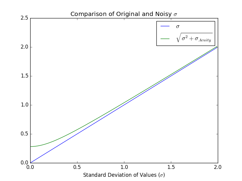
The plot basically shows that for \(\sigma \lt 1\) there is less than 1% difference between the original and noisy \(\sigma\), but for small values the difference increases as the original value approaches 0.

To get a sense of how this impacts the expected correct guesses, I plotted the expected number of correct guesses for the numeric attribute \((P(A_i = V_{ij})^2)\) for the three possible approaches: unbounded \(\sigma\), acuity bounded \(\sigma\), and noisy \(\sigma\):

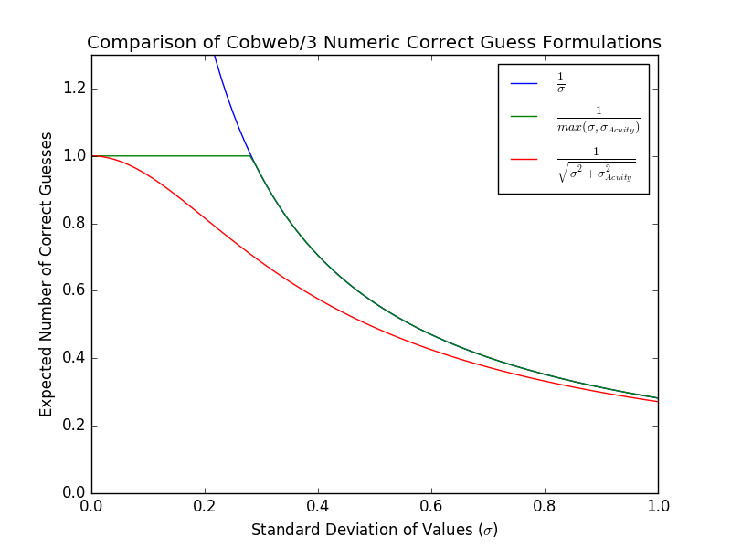
This graph shows that the unbounded version exceeds 1 correct guess as we get close to 0. This is bad when we have mixed numeric and nominal features because numeric features will worth more than the nominal features. Next, we see that the acuity bounded version levels off at 1 correct guess. This is also a problem because it makes it impossible for COBWEB to distinguish which values produce the best category utility for small values of \(\sigma\). The noisy version produces the most reasonable results: it provides the ability to discriminate between different values of \(\sigma\) for the entire range (even small values), it never exceeds 1 correct guess, and for medium and larger values of \(\sigma\) it produces the same behavior as the other approaches.

Problem 2: Sensitive to Scale of Variables

Additionally, COBWEB/3 is sensitive to the scale of numeric feature values. If feature values are large (e.g., 0-1000 vs 0-1), then the standard deviation of the values will be larger and it will have a lower number of expected correct guesses. To overcome this limitation, my implementation of COBWEB/3 performs online normalization of the numeric features using the estimated standard deviation of all values, which is maintained at the root of the categorization tree. My implementation normalizes all numeric values to have standard deviation equal to one half, which is maximum standard deviation that can be achieved in a nominal value. This ensures that numeric and nominal values are treated equally.

Evaluation of COBWEB/3 Implementation

In order to test whether my implementation of COBWEB/3 is functioning correctly and overcoming the stated limitations, I replicated the COBWEB/3 experiments conducted by Li and Biswas (2002). In their study, they created an artificial dataset with two numeric and two nominal features. Here is the approach Li and Biswas (2002) used to generate their 180 artificial datapoints:

The nominal feature values were predefined and assigned to each class in equal proportion. Nominal feature 1 has a unique symbolic value for each class and nominal feature 2 had two distinct symbolic values assigned to each class. The numeric feature values were generated by sampling normal distributions with different means and standard deviations for each class, where the means for the three classes are three standard-deviations apart from each other. For the first class, the two numeric features are distributed as (N(mu=4, sigma=1)) and (N(mu=20, sigma=2)); for the second class, the distributions were (N(mu=10, sigma=1)) and (N(mu=32, sigma=2)); and for the third class, (N(mu=16, sigma=1))and (N(mu=44, sigma=2)).

Given these three clusters Li and Biswas added non-Gaussian noise to either the numeric or nominal features. To add noise, some percentage of either the numeric or nominal features were randomly selected and given the values specified by the other clusters. To compute a clustering Li and Biswas trained COBWEB/3 using all of the examples then assigned cluster labels based on which child of the root the examples was assigned to. Next, Li and Biswas computed a misclassification score for each assignment. The misclassification count was computed using the following three rules:

1. If an object falls into a fragmented group, where its type is a majority, it is assigned a value of 1,
2. If the object is a minority in any group, it is assigned a misclassification value of 2, and
3. Otherwise the misclassification value for an object is 0.

For this calculation if more than three groups are formed by COBWEB/3, the additional smaller groups are labeled as fragmented groups.

Here is the graph of COBWEB/3’s misclassification count (taken Li and Biswas’s paper) for increasing amounts of noise to either the numeric or nominal features:

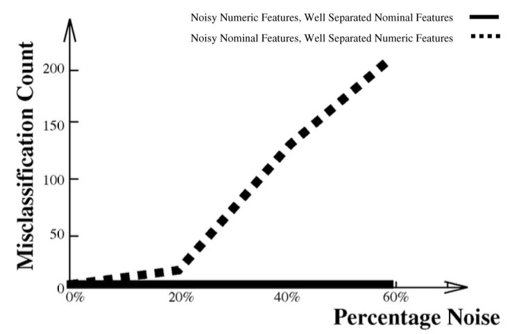
We can see from this graph that COBWEB/3 does not treat noise in the numeric and nominal features equally. Noise in the nominal values seems to have more of an impact on misclassification than noise in the numeric values. To ensure my implementation of COBWEB/3 is functioning normally after adding the new new approach for handling small values of \(\sigma\), I shut off normalization at the root and attempted to replicate Li and Biswas’s results. Here is a graph showing the performance of my implementation:

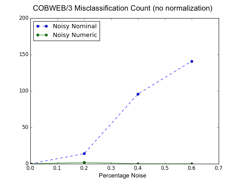
At a rough glance, it seems like both implementations are performing the same. Looking a little closer, my implementation has less misclassifications overall (max of ~140 vs. ~200). So it looks like the new treatment of \(\sigma\) is working and maybe is even improving performance. However, it seems like my implementation is still giving preference to nominal features; i.e., noise in nominal features has a bigger impact on misclassification count. When reading the Li and Biswas paper, my initial thoughts were that the dispersal of the numeric values (e.g., std of the clusters are either 1 or 2) might cause COBWEB/3 to give less preference to numeric features because larger standard deviations of values correspond to a lower number of expected correct guesses (see the figure titled Comparison of COBWEB/3 Numeric Correct Guess Formulations). To test if this was the case, I activated online normalization of numeric attributes in my COBWEB/3 implementation and replicated the experiment. Here is the results of this experiment:

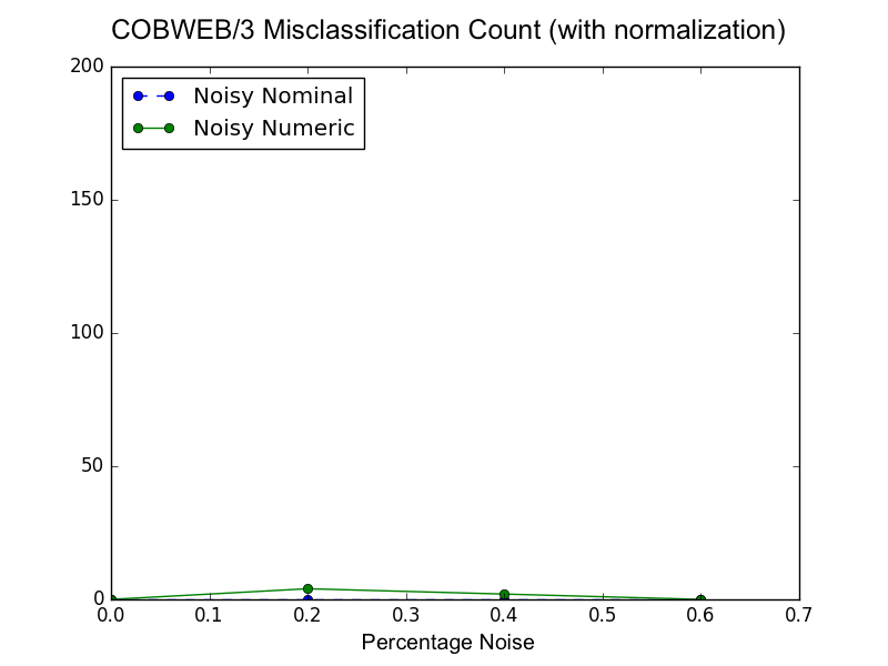
This result shows that COBWEB/3 with online normalization treats numeric and nominal attributes more equally. The original Li and Biswas paper compared COBWEB/3 to two other systems (AUTOCLASS and ECOBWEB) and to a new algorithm that they propose (SBAC). Their proposed algorithm was the only one that had better performance than COBWEB/3. When I looked at the implementation details, a key feature of their system is that is is less sensitive to the scale of attributes because it uses median splits. This last graph shows that my COBWEB/3 implementation performs as well (maybe better) than their proposed SBAC algorithm.

Conclusions

The COBWEB/3 algorithm provides a natural approach for doing machine learning with mixed numeric and nominal data. However, it has two problems: it struggles when the standard deviation of numeric attributes is close to zero and it is sensitive to the scale of the numeric attributes. Erik Harpstead and I created an implementation of COBWEB/3 (available on GitHub) that overcomes both of these issues. To handle the first issue we assume some measurement noise for numeric attributes that results in expected correct guess values that make sense (i.e., no more than one correct guess can be achieved per numeric attribute) and that provide the ability to discriminate between values of \(\sigma\) across the entire range \((0,\infty)\). To handle the second issue we added a feature for performing online normalization of numeric features. Next, I tested the modified version of COBWEB/3 by replicating an artificial noise experiment by Li and Biswas (2002). I showed that showed that modified COBWEB/3 is less sensitive to noise than the the original version of COBWEB/3 and treats numeric and nominal attributes more equally. These results show that my implementation of COBWEB/3 is an effective approach for clustering with mixed numeric and nominal data.