Modeling Student Learning in Python
An exploration of how to model human learing in a geometry tutor using the additive factors model (AFM) as well the extended model that accounts for slipping (AFM+S).
Problem Overview
Statistical models of student learning, such as the Additive Factors Model Cen, 2009), have been getting a lot of attention recently at educational technology conferences, such as Educational Data Mining. These models are used to estimate students’ knowledge of particular cognitive skills (e.g., how to compute the sum two numbers) given their problem-solving process data. The learned estimates can then be used to predict subsequent student performance and to inform adaptive problem selection. In particular, educational technologies, such as intelligent tutoring systems, can use these estimates to assign each student practice problems that target their specific weaknesses, so that they do not waste time practicing skills they already know. There is some evidence that the time savings with this approach is substantial (Yudelson and Koedinger, 2013); for example, studies have shown that students can double their learning in the same time (Pane et al., 2013) or learn more in approximately half the time (Lovett et al., 2008) when using an adaptive intelligent tutoring system.
Additionally, statistical models of learning can be used to identify the component skills that students are learning in a particular digital learning environment. A key element of these models is that researchers must label the steps of each problem with the skills that they believe are needed to correctly perform them. Researchers can then develop alternative skill models (also called knowledge component models, using the convention from Koedinger et al., (2012) and see which models result in an increased ability to predict the student behavior. The division between skills might not seem important, but is in fact crucial for adaptive problem selection in that it makes the adaptive selection more precise. When skills are too coarse, students spend time practicing sub-skills they don’t need to. Conversely, when they are too fine, students have to do additional work to prove that they know each skill when, in fact, multiple skills are actually just the same skill.
Given the usefulness of these models and their practical applications, a lot of work has been done to make it easier for researchers to develop new models (both statistical and skill). One resource that I constantly rely on for my research is DataShop, an online public repository for student learning data that (at the time of this writing) contains more than 193 million student transactions across 821 datasets. Further, the DataShop platform also implements the Additive Factors Model, a popular statistical model of student learning, so it is easy to start investigating learning in the available datasets.
While DataShop is capable of running the Additive Factors Model server side, there is no easy way to run the model on your local machine. This is an issue when I want to run different kinds of evaluation on the models that are not available directly in DataShop (e.g., different kinds of cross validation). It is also a problem when you have large datasets because DataShop will not run the Additive Factors Model if the dataset is too big. To overcome this issue some researchers have used R formulas that approximate the model (e.g., see DataShop’s documentation). However, these approximations don’t don’t take into account some of the key features of the Additive Factors Model, such as strictly positive learning rates. Additionally, it isn’t possible to use other variants of of the Additive Factors Model, such as my variant that adds slipping parameters (MacLellan et al., 2015); i.e., it models situations where students get steps wrong even when they correctly know the skills, which is a key feature in other statistical learning models such as Bayesian Knowledge Tracing.
To address this issues I implemented both the standard Additive Factors Model (AFM) and my Additive Factors Model + Slip (AFM+Slip) in Python. Further, I wrote the code so that it accepts data files that are in DataShop format (thanks to Erik Harpstead, we should be able to support both transaction-level and student-step-level exports). The code, which I am tentatively calling pyAFM, is available on my GitHub repository. In this blog post, I briefly review these two models that I implement (AFM and AFM+Slip) and provide an example of how they can be applied to one of the public datasets on DataShop.
Background
The Additive Factors Model, and other students models such as Bayesian Knowledge Tracing (Corbett & Anderson, 1994), extend traditional Item-Response Theory models to model student learning (IRT only models item difficulty and student skill). A key component of these modeling approaches is something called a Q-Matrix (Barnes, 2005), which is mapping of student steps to the skills, or knowledge components, needed to solve them . An initial mapping is typically based on problem types. For example, all problems in the multiplication unit might be labeled with the multiplication skill. Another common initial mapping is to assign each unique step to its own skill (this is basically what most IRT models do). However, good mappings can be difficult to find and often require researchers to iteratively test mappings to see which better fits the student data. Approaches that utilize Q matrices and that model learning typically fit the data substantially better than simple regression models based on problem type alone, such as the technique discussed in this Khan Academy blog post, because they take the effects of different component skills and learning into account.
Additive Factors Model
Many student learning models have been proposed that utilize Q matrices and that model learning, but I’ve chosen to focus on the Additive Factors Model, which is one of the more popular models. The Additive Factors Model is a type of logistic regression model. As such, it assumes that the probability that a student will get step i correct (\(p_i\)) follows a logistic function:
\[p_i = \frac{1}{1 + e^{-z_i}}\]
In the case of Additive Factors Model,
\[z_i = \alpha_{student(i)} + \sum_{k \in KCs(i)} (\beta_k + \gamma_k \times opp(k, i))\]
where \(\alpha_{student(i)}\) corresponds to the prior knowledge of the student who performed step i, \(KCs(i)\) specifies the set of knowledge components used on step i (from the Q-matrix), \(\beta_k\) specifies the difficulty of the knowledge component k, \(\gamma_k\) specifies the rate at which the knowledge component k is learned, and \(opp(k, i)\) is the number of practice opportunities the student has had on knowledge component k before step i. Here is an annotated visual representation of the learning curve predicted by the Additive Factors Model:
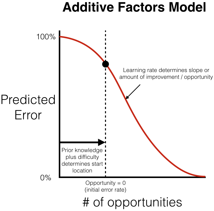
The Additive Factors Model, as specified by Cen and DataShop, also has two additional features. First, the learning rates are restricted to be positive, under the assumption that practice can only improve the likelihood that a student will get a step correct. Second, to prevent overfitting an L2 regularization is applied to student intercepts. These two features are left out in most implementations of the Additive Factors Model because they cannot be easily be implemented in most logistic regression packages.
To implement the Additive Factors Model, I implemented my own Logistic Regression Classifier (on my GitHub here). For convenience, I implemented my classifier as a Scikit-learn classifier (so I can more easily use their cross validation functions). I couldn’t just use Scikit-learn’s logistic regression class because it didn’t provide me with the ability to use box constraints (i.e., to specify that learning rates most always be greater than or equal to 0). Their implementation also does not allow me to specify different regularization settings for individual parameters (i.e., to only regularize the student intercepts). My custom logistic regression classifier implements this functionality.
Additive Factors Model + Slip
This model extends the previous model to include slipping parameters for each knowledge component. These parameters are used to account for situations where a students incorrectly apply a skill even though they know it. To add these parameters to the model I had to extend logistic regression to include bounds on one side of the logistic function (an approach I call Bounded Logistic Regression in my paper). Now, the probability that a student will get a step i correct (\(p_i\)) is modeled as two logistic functions multiplied together:
\[p_i = \frac{1}{1 + e^{-s_i}} \times \frac{1}{1 + e^{-z_i}}\]
Identical to the previous model,
\[z_i = \alpha_{student(i)} + \sum_{k \in KCs(i)} (\beta_k + \gamma_k \times opp(k, i))\]
Additionally, the slipping behavior is modeled as, \[s_i = \tau + \sum_{k \in KCs(i)} \delta_k \] where \(\tau\) corresponds to the average slip rate of all knowledge components and \(\delta_k\) corresponds to the difference in slipping rate for the knowledge component k from the average. The logistic function is used to model the slipping behavior because in some situations steps are labeled with multiple knowledge components and the logistic function has been shown to approximate both conjunctive and disjunctive behavior when combining parameters (Cen, 2009). Here is what the predicted learning curve looks like after incorporating the new skipping parameters:
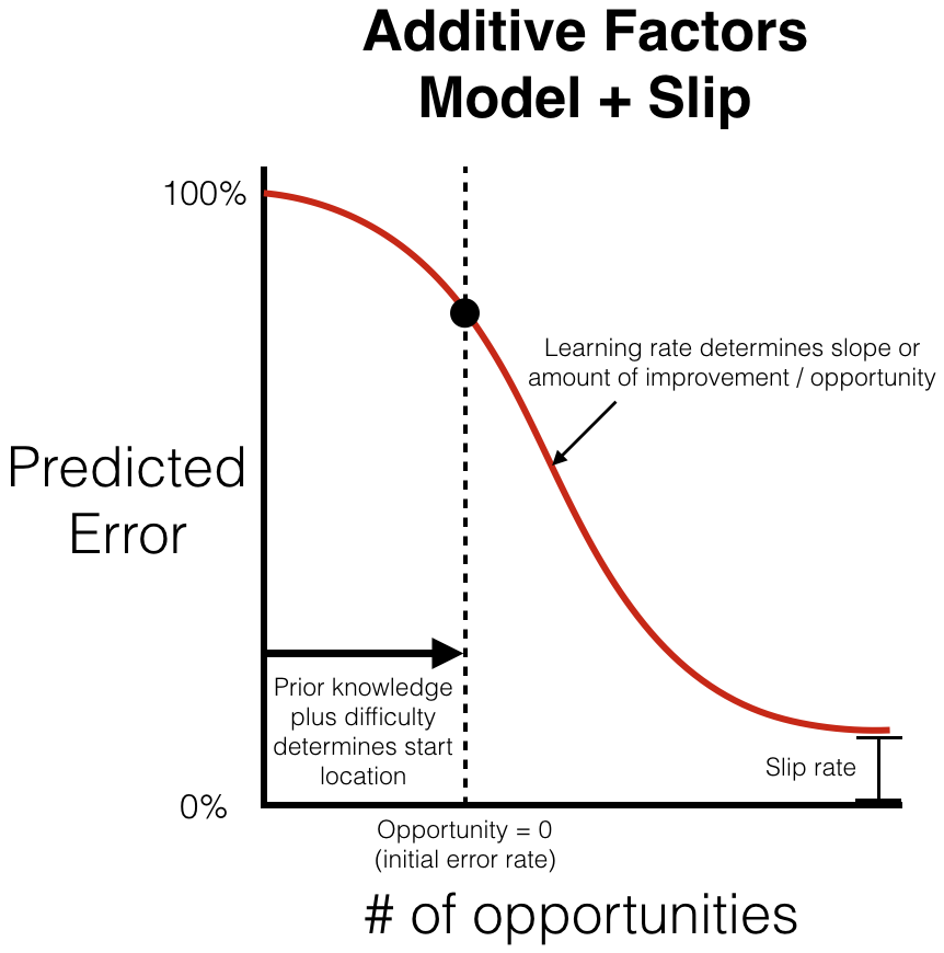
Similar to the previous model, this model also constrains the learning rates to be positive and regularizes the student intercepts. Additionally, it regularizes the individual student slip parameters (the (\delta)’s) to prevent overfitting.
In order to construct this model I implemented a Bounded Logistic Regression classifier (code is on my GitHub). This classifier is different from the traditional Logistic Regression in that it accepts two separate sets of features (one set for each logistic function).
Comparison on the Geometry Dataset
In my paper I tested this technique on five different datasets across four domains (Geometry, Equation Solving, Writing, and Number Line Estimation). For this blog post, I wanted to step through the process of running both models on the Geometry dataset and to highlight one situation where the two models differ in their behavior.
First, I went to DataShop and exported the Student Step file for the Geometry 96-97 dataset. Next, I ran my process_datashop.py script twice on the exported student step file (once for AFM and once for AFM+S). I selected the knowledge component model that I wanted to analyze (I chose the model LFASearchAICWholeModel3, which is one of the best fitting) and my code returned the following cross validation results (I only included the first three KC and Student parameter estimates for brevity):
$ python3 process_datashop.py -m AFM ds76_student_step_All_Data_74_2014_0615_045213.txt
 Unstratified CV    Stratified CV    Student CV    Item CV
-----------------  ---------------  ------------  ---------
            0.397            0.400         0.410      0.402
KC Name                                                             Intercept (logit)    Intercept (prob)    Slope
----------------------------------------------------------------  -------------------  ------------------  -------
Geometry*Subtract*Textbook_New_Decompose-compose-by-addition                    2.563               0.928    0.000
Geometry*circle-area                                                           -0.236               0.441    0.171
Geometry*decomp-trap*trapezoid-area                                            -0.536               0.369    0.091
...
Anon Student Id                         Intercept (logit)    Intercept (prob)
------------------------------------  -------------------  ------------------
Stu_bc7afcb7eef3ccfc1fc6547ed5fcde34               -0.316               0.422
Stu_c43d4a17398b2667daacdc70c76cf8ef               -0.055               0.486
Stu_4902934aaa88223a58cd80f44d0011e1               -0.017               0.496
...
$ python3 process_datashop.py -m AFM+S ds76_student_step_All_Data_74_2014_0615_045213.txt
Unstratified CV    Stratified CV    Student CV    Item CV
-----------------  ---------------  ------------  ---------
            0.396            0.397         0.409      0.399
KC Name                                                             Intercept (logit)    Intercept (prob)    Slope    Slip
----------------------------------------------------------------  -------------------  ------------------  -------  ------
Geometry*Subtract*Textbook_New_Decompose-compose-by-addition                   17.573               1.000    0.745  -0.592
Geometry*circle-area                                                           -1.098               0.250    0.194   0.172
Geometry*decomp-trap*trapezoid-area                                            -1.386               0.200    0.106  -0.288
...
Anon Student Id                         Intercept (logit)    Intercept (prob)
------------------------------------  -------------------  ------------------
Stu_bc7afcb7eef3ccfc1fc6547ed5fcde34               -0.307               0.424
Stu_c43d4a17398b2667daacdc70c76cf8ef               -0.007               0.498
Stu_4902934aaa88223a58cd80f44d0011e1                0.174               0.543
...
These results show that for the this dataset the AFM+S model performs better on cross validation than the AFM model (for all types of cross validation). It is also interesting to note that the difficulties of the skills are different after taking the slipping into account. The student prior knowledge estimates are also different. This makes sense because the initial difficulty and prior knowledge estimates are being adjusted to account for the slipping rates. It is also important to note that the learning rate estimates are much higher in the AFM+S model. To get a better sense for why, I plotted the learning curves from the student data with the associated predicted learning curves from the two models. To do this I used my plot_datashop.py script (when prompted I selected the LFASearchAICWholeModel3 KC model) :
$ python3 plot_datashop.py ds76_student_step_All_Data_74_2014_0615_045213.txt
This returns an overall learning curve plot for all of the knowledge components together and a plot of the learning curve for each individual knowledge component. Here is the overall learning curve:
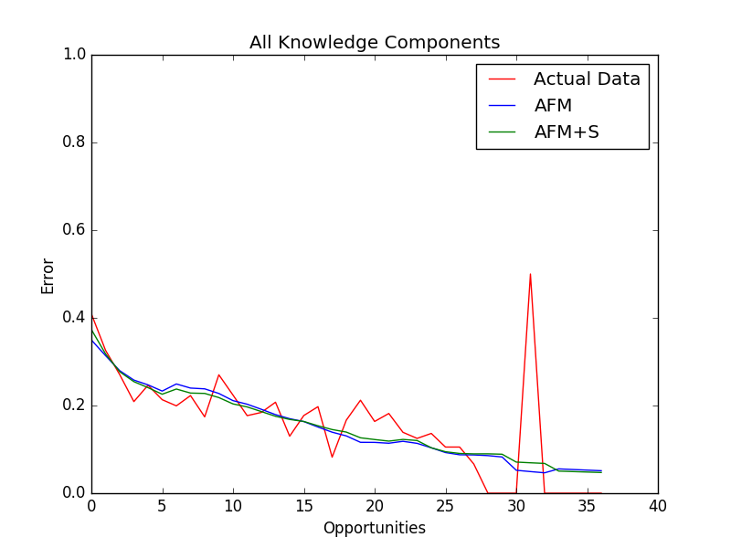
It is a little hard to to see differences between the two models, but one thing to point out is that the AFM+S model better fits the steeper learning rate at the beginning. This would agree with my finding that the learning rates in the AFM+S model tend to be higher than the AFM model. This effect is much more pronounced if we choose knowledge component where the error rate does not converge to zero. For example, lets look at the Geometry*compose-by-multiplication skill:
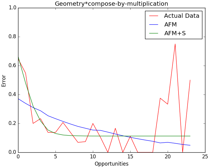
We can see from this graph that the traditional additive factors model is trying to converge to zero error, so higher error rates in the tail cause it to have a shallower learning rate at the beginning. In contrast, the model with the slipping parameters better models the initial steepness of the learning curve, as well as the higher error rate in the tail.
Summary
I implemented the Additive Factors Model and Additive Factors Model + Slip in Python and showed how it can be used to model student learning in a publicly available dataset from DataShop. My hope is that by making AFM and AFM+S available and easy to run in Python, more people will consider using it (Hey you over at Khan Academy!). Also, as a researcher, I know how much of a pain it is to have to implement someone else’s student modeling technique, just to compare your technique to it. Now other researchers can easily compare their student learning model to the Additive Factors Model (with all of its nuances, such as positive learning rates and regularized student intercepts) as well as to my Additive Factors Model with Slipping parameters. I’d welcome people showing that their technique is better than mine, just remember to cite me :).